We work with a synthetic 3D figure-eight throughout: two loops joined at a single saddle, ~600 points, dense on the lobes and sparse near the crossing. The shape exercises every part of the pipeline — two H1 classes (one per loop), several H0 basins, a real geometric saddle, and heterogeneous sampling density. Simpler shapes drop at least one of these ingredients (a torus has only one H1 class, two Gaussian basins have no H1 at all, a single annulus has no saddle), which is why we picked this one.
Reading the cloud's local sampling scale
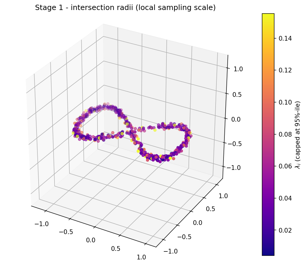
The very first thing the algorithm does is line the points up in a farthest-point permutation: at each step pick the point that maximises the minimum distance to the prefix already chosen. The distance to the nearest point in the prefix at the moment a new point is added is its intersection radius λi — a per-vertex local sampling scale. Small λ means crowded neighbourhood; large λ means sparse or outlier.
On the figure-eight you can watch the algorithm visibly hop between the two lobes as the prefix grows, and the resulting λ-coloured cloud shows the dense-on-lobes / sparse-near-the-crossing pattern that all downstream stages will key off:
Throwing away most candidate edges
With a per-vertex sampling scale in hand, the next move is to decide
which edges of the complete graph on the cloud are even worth keeping.
A naive Rips construction at scale α admits every edge with d(p,q) ≤ 2α — O(N²) of them, most of which are redundant in
the sense that they thicken already-dense regions without adding
anything topologically new. The ε-sparsifier admits only edges whose
scale α fits the per-vertex perturbation bands set by λp,
λq, ε; edges that exceed min(λp, λq) / [ε(1−ε)]
get dropped entirely. Sheehy (2013) shows the resulting filtration's
persistence diagram is within (1+ε) of the full Rips' diagram, so the
savings are essentially free.
Sweeping ε from aggressive (0.5) up to lenient (0.99), you can watch the sparsifier loosen its grip — at small ε most edges are pruned, at ε near 1 most survive:
Turning density into a height function
The surviving vertices and edges now need filtration values — the
scale α at which each will enter the simplicial complex. Every
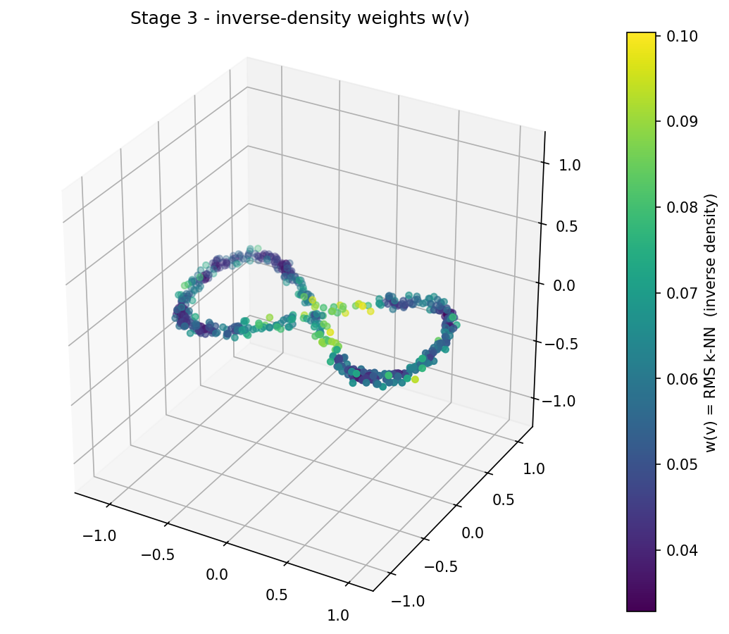
surviving vertex gets an inverse-density weight w(v) = √( (1/k) Σ d(v, kNNj)² ): the
root-mean-square distance to its k nearest neighbours. Dense
neighbourhood gives small w, sparse neighbourhood gives large w. We
treat this number as the vertex's filtration value α(v) = w(v),
which means dense vertices enter the filtration first — the densest-first rule.
Painted on the figure-eight, this is the inverse-density landscape the rest of the pipeline will sweep through: the lobes (dense) sit low, the crossing region (sparse) sticks up:
Edges and triangles inherit their α from the same density picture.
Imagine each vertex as a "bubble" of radius w(v); as a single global
scale α grows, each bubble inflates to radius √(α² − w(v)²). An edge is born the moment its two
endpoints' bubbles just touch. A triangle is born at the α of its
last-born edge.
In one line: α(e) is the time on the α-clock at which edge e joins the simplicial complex (which is when the "touch" happens). Concretely:
where d = d(vi, vj) is the metric distance. The vertex weight w(v) is the RMS distance to v's k nearest neighbours. The edge formula is the closed form for "two density-inflated balls just touch", with a clamp ensuring α(e) is never smaller than either endpoint's α. A triangle is born at the α of its latest-born edge — equivalently, when its third edge enters the complex.
Milestone — the SWR 1-skeleton is fully formed here. Every surviving edge has its α(e), every triangle has its α(t), and the simplicial complex is a single sorted-by-α event log on disk. Everything after this section reads that log; nothing after this section adds new simplices to it.
Replaying the growth as a persistence diagram
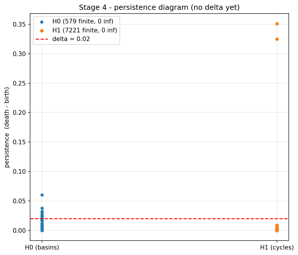
Run the growth on the figure-eight and you get a continuous sweep that vacuums up the cloud bottom-first — basins fill long before ridges, and the loops only close at the very end when the triangles supporting them finally appear. The persistence step replays that log and bookkeeps births and deaths: vertices create new connected components, edges merge components (a younger component dies into an older one), and triangles fill loops. Each merge or fill becomes one persistence pair with a measurable lifetime death − birth. On the figure-eight you can see two stand-out H1 pairs in the resulting diagram (the two lobes), several H0 pairs (the basins), and a cluster of short pairs near the diagonal that are clearly noise — and crucially this stage does no thresholding, so every feature, however trivial, is in the diagram:
Cancelling noise and tracing the skeleton
Only at the very last step does the persistence threshold δ enter the picture. The Forman cancellation rule says: every persistence pair with lifetime ≤ δ is treated as noise (the birth and death simplices are matched and erased); every pair with lifetime > δ survives as critical. The algorithm then walks descending gradient flows between surviving critical 1-simplices (saddles) and critical 0-simplices (basin minima), and writes those traced flows as the edges of the discrete-Morse skeleton GM.
Sweeping δ on the figure-eight makes this concrete. At small δ the skeleton is dense and noisy; as δ grows, noise pairs cancel first, then shallower basins, until eventually only the most persistent loop survives:
Milestone — the discrete-Morse skeleton GM is fully formed here. It is a strict subgraph of the SWR 1-skeleton: only the edges along the traced descending V-paths between surviving critical simplices survive. From this point on, TopoMimic analyses GM directly — extracting fundamental cycles (DM-cycles, H1) and edge-disjoint paths between persistent minima (DM-paths, H0).
Three things easy to confuse
- SWR 1-skeleton ≠ discrete-Morse skeleton. The former is the full ε-sparsified Rips edge set (thousands of edges), the substrate the topology engine operates on. The latter is its post-cancellation V-path-traced subgraph (dozens of edges) and is what TopoMimic analyses.
- The PCD path is not a lower-star filtration. Lower-star is the baseline branch of the dmpcd library (Gaussian KDE on a fixed-radius Rips, with simplex α = max(f(vertices))). The PCD branch uses the closed-form weighted-Rips birth from Stage 3 — different filtration rule, different persistence binary.
- δ is read only by the last binary. Persistence is δ-agnostic. You can sweep δ post-hoc with the same persistence diagram — no need to recompute the filtration or the persistence.