Behaviors are where a trajectory lingers. Transitions are what is missing.
How an animal moves from one behavior to the next, walking into a rear or a rear into a turn, is a central question in neuroethology. Yet the standard tools describe transitions only after a coarse-graining. An autoregressive HMM such as Keypoint-MoSeq assigns every frame a syllable and summarizes transitions as a matrix over syllables. A variational autoencoder partitions a latent embedding. Mapper builds a graph over overlapping density patches. In each case the states come first, and a transition is whatever lies between two of them, at whatever resolution the state assignment allows.
We take the opposite view. In a suitable feature space a sustained behavior is a dense region of the trajectory: the animal spends many frames there. A transition is the sparse corridor or loop that connects dense regions: the trajectory passes through it quickly and rarely. That structure belongs to the shape of the density landscape, a region of the space shaped by what is missing, so it can be read off directly with topology and should look the same in different coordinates.
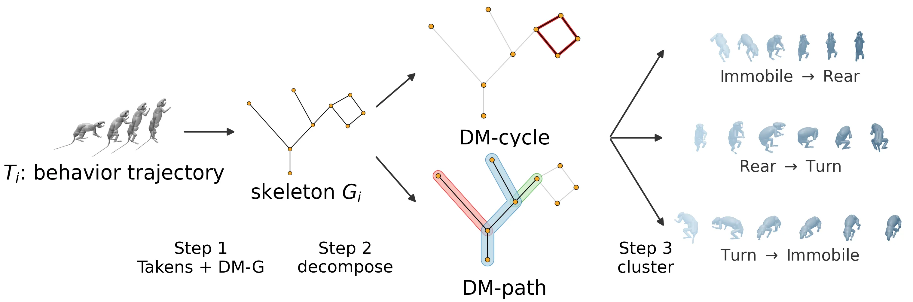
A trajectory is Takens-embedded and skeletonized into a discrete-Morse graph (Step 1), decomposed into DM-cycles (H₁ loops) and DM-paths (the split tree) (Step 2), and the pooled primitives are clustered under the 2-Wasserstein distance into behavioral transition clusters (Step 3). The rest of this page walks through each step with the data behind it.
This page walks through what we did, with the rollouts behind the paper’s figures rendered as video and the key constructions made interactive.
A rat, a physics simulator, and three ways to describe it
The trajectories come from MIMIC-MJX. Markerless 3D motion capture of a freely moving rat is fit by inverse kinematics to a biomechanical model, and a deep reinforcement learning policy is trained to imitate the resulting motion in the MuJoCo physics simulator. At each step an encoder maps a short window of the upcoming reference to a 16-dimensional latent intention, and a decoder combines it with proprioception to produce the actions that drive the body.
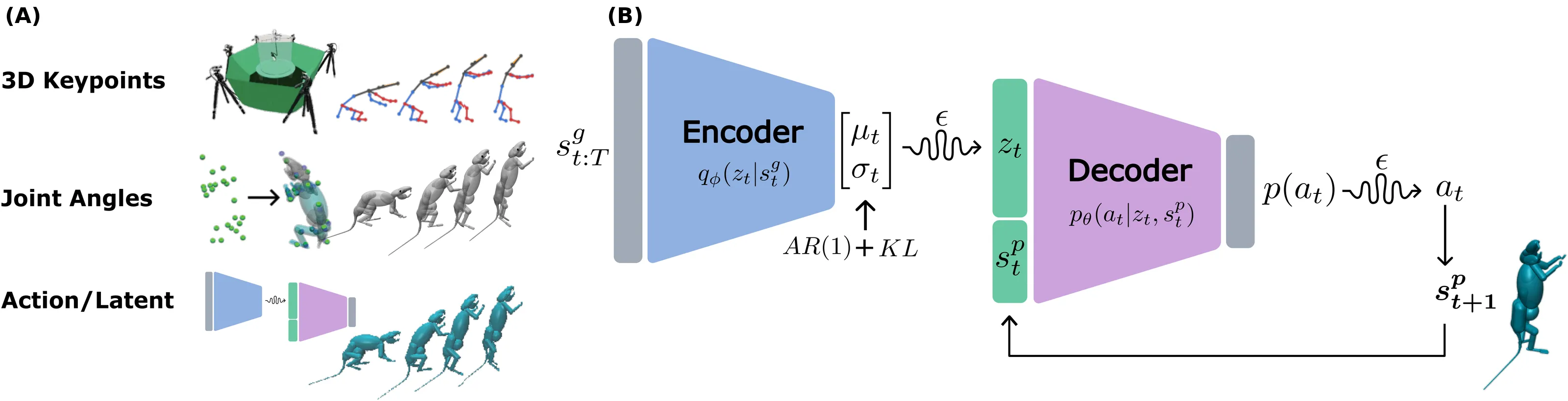
The MIMIC-MJX pipeline (Zhang et al., 2025). (A) Motion capture is fit to a biomechanical model and a policy learns to imitate it. (B) The encoder maps the reference window to the latent intention; the decoder turns intention and proprioception into action.
The same 842 clips (about 500 frames each at 30 Hz) are analyzed in three representations at increasing levels of abstraction:
- Egocentric keypoints (ekp, 60-d): the 20 tracked keypoints in a body-fixed frame. Where the body is.
- Joint angles (qpos, 67-d): the rolled-out joint configuration with the global root pose removed. How the body is posed.
- Intention (16-d): the policy’s learned latent, drift-invariant by construction. What change drives the body toward its next pose.
Intention and joint angles are spaces a keypoint segmenter cannot offer, and they matter here for a geometric reason: a skeleton only forms where behaviorally similar frames recur near each other. Uncorrected drift pulls repeated instances of the same behavior apart, so we expect the cleanest structure in intention and qpos and the weakest in ekp.
The behaviors, and the transitions between them
To evaluate, and only to evaluate, every frame carries a behavior label (Walk, Immobile, Turn, Rear) and a turn direction (left, right, straight), produced by an open-source heuristic labeler and proofread by two annotators. Below is one instance of each of the twelve directed transitions, rendered from the policy rollouts in the simulator.
The video counterpart of the paper’s Figure 5. Each clip replays one representative ground-truth transition at half speed under the paper’s shared camera. The amber body is live; the six poses of the static figure are dropped into the scene, light to dark, as the body passes them, and the final held frame is the paper’s panel. The strip at the bottom is the ground-truth behavior over the window (tick marks are the six poses). Instances are chosen as in the paper: each side of the labeled boundary is scored against the kinematic signature of its own label (speed, yaw rate, torso height), and the instance whose weaker side scores best is shown. n is the number of instances of that transition in the dataset. Click a clip to enlarge it.
Purely rotational transitions (Turn → Immobile, Immobile → Turn) are the hardest to see from one viewpoint: the heading changes while the body stays in place.
How the method works
The pipeline has three steps. The first two run on each clip separately and turn it into a handful of topological primitives; the third pools the primitives from all clips and clusters them.
Each recorded clip becomes a point cloud in a feature space. Its discrete-Morse skeleton traces the ridges of the cloud's density, and two kinds of structure are cut from it: DM-cycles, loops whose way out and way back differ, and DM-paths, corridors between dense behavioral regions.
Primitives from all clips are pooled and clustered under the 2-Wasserstein distance. Each cluster is a candidate behavioral transition. No state partition is fit anywhere, and ground-truth labels are used only to evaluate the clusters afterwards.
Pick a tab to light up the modules active in each step. The right panel shows each step on the animal itself, using one real clip (clip 447: Rear, Walk, Rear) and its stored intention-space outputs. Takens: the pose now with the poses τ and 2τ frames earlier, which together form one point of the cloud. DM skeleton: the body tinted by the k-NN inverse density of that point. Primitives: each stored DM-cycle and DM-path of the clip, replayed. W2 clustering: three real DM-cycles from the paper’s DMC-Int clustering (seed 0) with their exact W₂² distances.
Why a skeleton holds the transitions
The discrete-Morse graph reconstruction we build on was developed to recover road networks from noisy GPS samples, and that two-dimensional setting is the easiest place to see what it does. Points sampled around a hidden graph induce a density field. Viewed as a terrain, the hidden roads are its mountain ridges: formally the 1-stable manifolds, the integral lines that connect density peaks through saddles. Estimating them directly is fragile, so the construction works with discrete Morse theory on a simplicial complex over the points and uses persistent homology to cancel ridges that are not significant, under a threshold δ.
Below is that construction run for real (for a stage-by-stage account of the algorithm itself, see the PCD walkthrough). The point cloud and terrain are the road network of the paper’s Figure 3A; the red graph is the raw output of the same discrete-Morse backend we use on trajectories, recomputed at each δ.
Drag to rotate. The slider sets the persistence threshold δ; each position is a separate run of the backend (k = 5) on the same 796 points. Up to δ = 0.35 the recovered graph keeps three independent loops (the two diamonds plus one small noise loop) and every outward branch; at δ = 0.5 only the two diamonds remain as loops, at δ = 0.8 one, and at δ = 1.2 everything has been cancelled. The “DM-cycles + DM-paths” view decomposes each recovered graph exactly as Step 2 does on trajectories. Toggle “hidden graph” to compare with the roads the points were sampled from.
On a trajectory the same logic applies, with behaviors in place of junctions. Frames of a sustained behavior pile up into a density peak; the frames where the body reconfigures from one behavior to the next are few and spread out, so they form a low-density ridge between peaks. The skeleton is that set of ridges, and Step 2 cuts it into two kinds of piece.
A DM skeleton: a split tree with one loop attached. Height is density f; peaks are dense behavioral regions.
- DM-path · peak c dies at saddle 2
- DM-path · peak a dies at saddle 1
- DM-path · essential: global max to global min
- DM-cycle · the loop (minimum cycle basis)
The synthetic skeleton of the paper’s Figure 3B (a split tree plus one loop), decomposed step by step. The DM-cycle is the H₁ loop: a recurrence where the trajectory leaves a region and returns by a different route. Because every point of a Takens cloud is a short window of motion, that recurrence is one of dynamics, so a gait closes a loop without ever passing through a common pose. DM-paths are the persistence pairs of the remaining split tree, read as transition corridors. This is standard 0-dimensional persistence on a tree; what is ours is the reading of each pair as a corridor.
What the discovered clusters look like
Pooled over all clips, the primitives are compared as distributions under the 2-Wasserstein distance and clustered (Step 3). The baselines assign every frame a discrete label, a syllable or a Mapper node, so their transition units are ordered pairs of consecutive sustained labels. Below are clusters from the four variants of the paper’s main comparison. Within a cluster, the two members should trace the same gross movement.
The video counterpart of the paper’s Figures 10 to 13 (seed 0). The title of each cluster is its majority-vote ground-truth label; each figure shows up to six uniquely labeled transition clusters and two members per cluster. Members are chosen as in the paper: the first 14 members of a cluster are scored on whether both labeled behaviors appear in order and on how few frames belong to neither, with a penalty for members too spread out to fit the shared camera, and the best two are shown. Each video plays a member from its first to its last frame (for DM primitives, through the end of the last Takens window), with the paper’s six poses dropped as the amber body passes them; long members are played faster, at the speed noted on the clip. *Ours.
The baselines’ units are often long: a Keypoint-MoSeq pair can span most of a 500-frame clip, because a transition is the boundary between two sustained syllables. A DM primitive is a few seconds of behavior (on average 62 to 191 frames, depending on primitive and space), cut where the skeleton says the trajectory changes.
How much transition information survives the coarse-graining
Every method turns a clip into a per-frame label T: a primitive index for ours, a pair type for the baselines. We ask how much that label tells about the directed transition class Y each frame belongs to, by the mutual information I(T;Y), and place every configuration on the Information Bottleneck plane against its capacity H(T).
| variant | I(T;Y) | AMI |
|---|---|---|
| DMP-Qpos* | 0.895 | 0.230 |
| DMC-Intention* | 0.873 | 0.212 |
| KPMS-KP | 0.525 | 0.159 |
| DMP-Intention* | 0.510 | 0.172 |
| DMC-Qpos* | 0.474 | 0.166 |
| DMP-Ekp* | 0.363 | 0.163 |
| Mapper-Qpos | 0.322 | 0.121 |
| KPMS-Int | 0.286 | 0.108 |
| Mapper-EKP | 0.276 | 0.110 |
| DMC-Ekp* | 0.234 | 0.123 |
| Mapper-Int | 0.155 | 0.080 |
Baselines: mean over 3 seeds. DM decomposition is deterministic. H(Y) = 2.67 bits bounds I(T;Y).
The paper’s Figure 2 and Table 8, interactive. One dot per (method, seed); hover for values, click a family to hide it, switch the y axis to the cardinality-corrected AMI. DM decomposition is deterministic, so DM variants have one dot each.
DM cycles and paths in intention and qpos reach the top of the plane. The qpos DM-path carries the most transition information of any method, 0.90 bits, against 0.53 for the strongest baseline, Keypoint-MoSeq on keypoints, with intention DM-cycles close behind at 0.87. Correcting for label cardinality the lead is AMI 0.23 against 0.16; Mapper and Keypoint-MoSeq on intention stay at AMI ≤ 0.12. The ordering within DM, intention ≈ qpos > ekp, is the one the drift argument predicts.
Alignment, coherence and warping
Do the discovered clusters match the annotated transitions frame by frame? Each family is represented by its highest-information variant. Both DM variants align closest to the annotated boundaries on average, 0.04 to 0.06 below Keypoint-MoSeq and 0.01 to 0.03 below Mapper in mean DTW, but per row the picture is less one-sided: the DM columns win 6 of the 11 DTW rows. The warping decomposition separates the cases. The DM columns have the lower non-diagonal fraction on 9 of 11 rows and the higher sync ratio on 9 of 11; Keypoint-MoSeq leads on neither. Where Keypoint-MoSeq approaches our DTW, it does so by stretching a primitive onto the annotated window.
Frame-level alignment to the annotated window under a monotone time correspondence.
| Transition | DMC-Int* | DMP-Qpos* | Mapper-Qpos | KPMS-KP |
|---|---|---|---|---|
| Immobile → Rear [L] | — | 0.854 | — | 0.831 |
| Rear → Immobile [L] | — | 0.855† | 0.879 | 0.855 |
| Immobile → Rear [R] | — | 0.880† | — | 0.848† |
| Immobile → Rear [S] | 0.934 | 0.892 | 0.895 | 0.967 |
| Rear → Immobile [S] | 0.863† | — | 0.856 | 0.877 |
| Immobile → Turn [L] | 0.809 | 0.788 | 0.801 | 0.770 |
| Turn → Immobile [L] | 0.740 | 0.721 | 0.790 | 0.849† |
| Immobile → Turn [R] | 0.759 | 0.756† | 0.715† | 0.747 |
| Immobile → Walk [L] | 0.759† | — | — | — |
| Rear → Turn [L] | 0.826 | 0.778 | 0.818 | 0.918 |
| Turn → Walk [L] | 0.643 | — | — | — |
One variant per family, chosen by transition information. Bold = best in the row among populated cells. — = not discovered. † = one seed only. Direction tags: [L] left, [R] right, [S] straight. *Ours.
Paper Table 1. All metrics are computed in the same root-stripped joint-angle space. Per-variant grids for all twelve variants are in the paper’s appendix.
On KID, which ignores frame order and cannot warp, intention DM-cycles trail Keypoint-MoSeq by 13%, and we claim no distributional advantage. KID rewards breadth: a Keypoint-MoSeq cluster holds a median of about 14,000 frames against 3,800 for qpos DM-paths, sampling the window more fully while being markedly less coherent. Coverage is comparable: intention DM-cycles reach 10 of the 16 discovered directed transitions, against 11 for Mapper on intention and 9 for Keypoint-MoSeq on keypoints. The families are not nested. Four transitions, among them Walk → Turn [L] and Walk → Immobile [S], are found only by DM primitives, and Rear → Immobile [R] only by Mapper.
Three controls rule out simpler explanations. None of 110 baseline variants, sweeping Keypoint-MoSeq stickiness and state count and Mapper lens and interval count, improves on the tuned baselines. A full-clip control that skips the decomposition does worse than both DM variants in alignment (0.888) and coherence (0.797), so the decomposition, not the Wasserstein clustering, recovers the transitions. And DTW varies by at most 0.03 across the k-NN parameter in every space.
Citation
@inproceedings{bian2026shaped, title = {Shaped by What's Missing: Topological Invariance Simplification Discovers Behavioral Transitions}, author = {Bian, Kaiwen and Leonardis, Eric J. and Yang, Yuanjia and Zhang, Charles and Wang, Yusu and Pereira, Talmo D.}, booktitle = {Proceedings of the NeurIPS Workshop on Symmetry and Geometry in Neural Representations (NeurReps)}, series = {Proceedings of Machine Learning Research}, year = {2026}}The trajectories come from MIMIC-MJX. The discrete-Morse reconstruction uses PCD-Graph-Recon-DM (Magee and Wang, 2022). Baselines use Keypoint-MoSeq and tda-mapper.